Bootstrap confidience intervals with standard errors. bootstrap resamples dataset (e.g. diffusion coefficients) to calculate confidience intervals for a statistic measure of dataset.
bootstrap(fittedObj,n.reps=100)
Arguments
| n.reps | number of replicates for bootstrapping |
|---|---|
| fittedObj | output from fitNormDistr |
Value
Fit results from fitNormDistr that was used as the input for the function
Bootstraps results from bootstrapping. mean values of each samples, standard error for the mean, lambda
Details
A wrapper of boot::boot and mixtools::boot.se adapted for data format in sojourner package. Also returns stderr information by running boot.se from mixtools and an additional method for one-component distribution calculates the stderr separately. For multi-component distributions, the boot.se function from the mixtools package was used. For single-component distributions, a separate function was used to calculate the stderr and confidence interval.
Examples
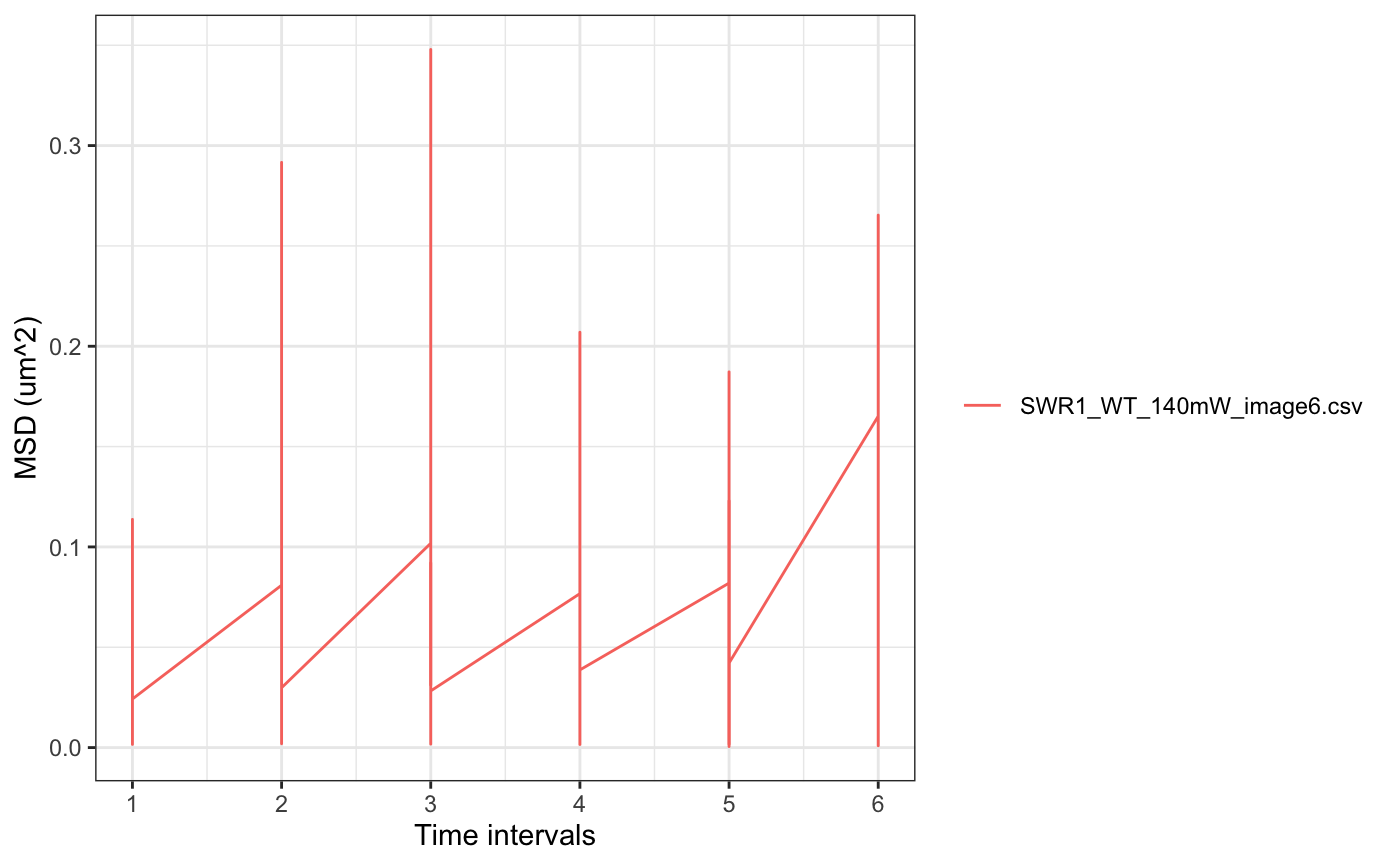
# read in track files folder=system.file('extdata','SWR1',package='sojourner') trackll=createTrackll(folder=folder, input = 3)#> #> Reading ParticleTracker file: SWR1_WT_140mW_image6.csv ... #> #> mage6 read and processed. #> #> Process complete.#> applying filter, min 5 max Inf#> applying filter, min 7 max Inf #> 45 tracks length > & = 1 45 tracks length > & = 2 45 tracks length > & = 3 45 tracks length > & = 4 45 tracks length > & = 5 45 tracks length > & = 6 #> #> ...#> #> applying static,lag.start= 2 lag.end= 5 #> lag.start 2 lag.end 5 #> #> Applying r square filter... 0.8#> Warning: NaNs produced#> #> IMPORTANT: Ensure a seed has been manually set! See help docs for more info. #> #> components analysis #> bootstrapping LRTS ... #> | | | 0% | | | 1% | |= | 1% | |= | 2% | |== | 2% | |== | 3% | |== | 4% | |=== | 4% | |=== | 5% | |==== | 5% | |==== | 6% | |===== | 6% | |===== | 7% | |===== | 8% | |====== | 8% | |====== | 9% | |======= | 9% | |======= | 10% | |======= | 11% | |======== | 11% | |======== | 12% | |========= | 12% | |========= | 13% | |========= | 14% | |========== | 14% | |========== | 15% | |=========== | 15% | |=========== | 16% | |============ | 16% | |============ | 17% | |============ | 18% | |============= | 18% | |============= | 19% | |============== | 19% | |============== | 20% | |============== | 21% | |=============== | 21% | |=============== | 22% | |================ | 22% | |================ | 23% | |================ | 24% | |================= | 24% | |================= | 25% | |================== | 25% | |================== | 26% | |=================== | 26% | |=================== | 27% | |=================== | 28% | |==================== | 28% | |==================== | 29% | |===================== | 29% | |===================== | 30% | |===================== | 31% | |====================== | 31% | |====================== | 32% | |======================= | 32% | |======================= | 33% | |======================= | 34% | |======================== | 34% | |======================== | 35% | |========================= | 35% | |========================= | 36% | |========================== | 36% | |========================== | 37% | |========================== | 38% | |=========================== | 38% | |=========================== | 39% | |============================ | 39% | |============================ | 40% | |============================ | 41% | |============================= | 41% | |============================= | 42% | |============================== | 42% | |============================== | 43% | |============================== | 44% | |=============================== | 44% | |=============================== | 45% | |================================ | 45% | |================================ | 46% | |================================= | 46% | |================================= | 47% | |================================= | 48% | |================================== | 48% | |================================== | 49% | |=================================== | 49% | |=================================== | 50% | |======================================================================| 100% #> ------------------------------------------------------------- #> Bootstrap sequential LRT for the number of mixture components #> ------------------------------------------------------------- #> Model = V #> Replications = 999 #> LRTS bootstrap p-value #> 1 vs 2 2.206494 0.703 #> #> #> most likely components 1 at significant level 0.05 #>#> Warning: row names were found from a short variable and have been discarded#> auto binwidth = 0.2157974#> $SWR1_WT_140mW_image6.csv #> [,1] #> proportion 1.00000000 #> mean 0.32091361 #> sd 0.05036344 #> log.lik -0.99716894 #># bootstrap new datasets d.boot=bootstrap(fittedObj) # manually set the number of bootstrap samples to 50 d.boot=bootstrap(fittedObj, n.reps=50)